My last blog wasn’t so sexy, what with all the data cleansing, and no predictive modelling. But in this blog I do something really cool – I train a machine learning model to find the left ventricle of the heart in an MRI image. And I couldn’t have done it without all of that boring data cleansing. #kaggle @kaggle

Aside from being a really cool thing to do, there is a purpose to this modelling. I want to find the boundaries of the heart chamber, and that is much easier and faster to do when I remove distractions. Once I have found the location of the heart chamber, I can crop the image to a much smaller square.

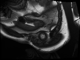
The input to the model will be a set of images. In order to simply what the model learns, I only gave it training images from sax locations near the centre of the heart.

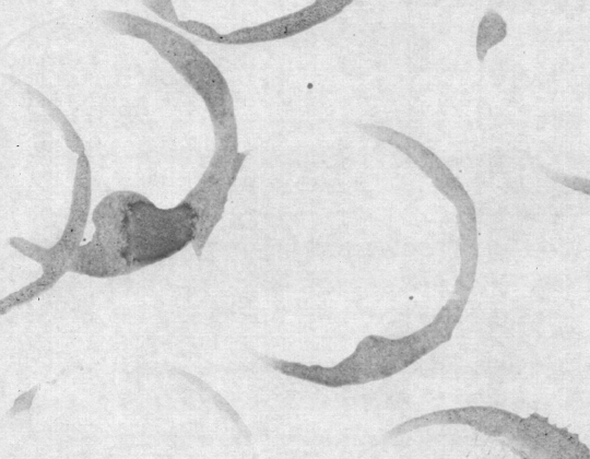
The output from the model will be the row number and column number of the centroid of the left ventricle heart chamber (the red dot in the images above).

I had to manually define those centroid locations for a training set of a few hundred of the images. This was laborious and time consuming, even after I automated some of the process. But it needed to be done, because otherwise the machine learning algorithm has no way of knowing what the true answers should be.

Even though I am much more comfortable coding in R than in Python, I used Python for this step because I wanted to use Daniel Nouri‘s nolearn library, which sits above lasagne and theano, and these libraries are not available in R. The convolution neural network architecture was based upon the architecture in Daniel Nouri’s tutorial for the Facial Keypoints Detection competition in Kaggle.

Step 1: Importing of all the Required Libraries

OK, so this part isn’t all that sexy either. But it’s the engine for all the cool modelling that is about to be done.

import numpy as np
import csv
import random
import math
import os
import cv2
import itertools
import math
import matplotlib.pyplot as plt
import pandas as pd
import itertools

from lasagne import layers
from lasagne.updates import nesterov_momentum
from lasagne.nonlinearities import softmax
from lasagne.nonlinearities import sigmoid
from nolearn.lasagne import BatchIterator
from nolearn.lasagne import NeuralNet
from nolearn.lasagne import TrainSplit
from nolearn.lasagne import PrintLayerInfo
from nolearn.lasagne.visualize import plot_loss
from nolearn.lasagne.visualize import plot_conv_weights
from nolearn.lasagne.visualize import plot_conv_activity
from nolearn.lasagne.visualize import plot_occlusion

%pylab inline
from lasagne.layers import DenseLayer
from lasagne.layers import InputLayer
from lasagne.layers import DropoutLayer
from lasagne.layers import Conv2DLayer
from lasagne.layers import MaxPool2DLayer
from lasagne.nonlinearities import softmax
from lasagne.updates import adam
from lasagne.layers import get_all_params
from nolearn.lasagne import NeuralNet
from nolearn.lasagne import TrainSplit
from nolearn.lasagne import objective

import theano
import theano.tensor as T

Step 2: Defining the Helper Functions

I used jupyter notebook as the development environment to set up and run my Python scripts. While there’s a lot to like about jupyter, one thing that annoys me is that print commands run in jupyter don’t immediately show text on the screen. But here’s a trick to work around that:

def printQ(s):
 print(s)
 sys.stdout.flush()

Using this helper function instead of the print function results in text immediately appearing in the output. This is particular helpful for progress messages on long training runs.

I like to use R’s expand.grid function, but it isn’t built in to Python. So I wrote my own helper function in Python that mimics the functionality:

def product2(*args, repeat=1):
 # product('ABCD', 'xy') --> Ax Ay Bx By Cx Cy Dx Dy
 # product(range(2), repeat=3) -> 000 001 010 011 100 101 110 111
 pools = [tuple(pool) for pool in args] * repeat
 result = [[]]
 for pool in pools:
 result = [x+[y] for x in result for y in pool]
 for prod in result:
 yield tuple(prod)

def expand_grid(dictionary):
 return pd.DataFrame([row for row in product2(*dictionary.values())],
 columns=dictionary.keys())

This next function reads a cleaned up image, checking that it has the correct aspect ratio, then resizing it to 96 x 96 pixels. The resizing is done to reduce memory usage in my GPU, and to speed up the training and scoring.

def load_image(path):
 # check that the file exists
 if not os.path.isfile(path):
   printQ('BAD PATH: ' + path)
 image = cv2.imread(path, cv2.IMREAD_GRAYSCALE)
 # ensure portrait aspect ratio
 if (image.shape[0] < image.shape[1]):
   image = cv2.transpose(image)
 # resize to 96x96
 resized_image = cv2.resize(image, (96, 96))
 # check that the image isn't empty
 s = sum(sum(resized_image))
 if np.isnan(s):
   print(path)
 return resized_image

My initial models were not performing as well as I would like. So to force the the model to generalise, I added some image transformations (rotation and reflection) to the training data. This required helper functions:

def rotate_image(img, degrees):
 rows,cols = img.shape
 M = cv2.getRotationMatrix2D((cols/2,rows/2),degrees,1)
 dst = cv2.warpAffine(img,M,(cols,rows))
 return dst

def transform_image(img, equalise, gammaAdjust, reflection, rotation):
 if equalise == 1:
   img = cv2.equalizeHist(img)
 if gammaAdjust != 1:
   img = pow(img / 255.0, gammaAdjust) * 255.0
 if reflection == 0 or reflection == 1:
   img = cv2.flip(img, int(reflection))
 if rotation != 0:
   img = rotate_image(img, rotation)
 return img

def transform_xy(x, y, equalise, gammaAdjust, reflection, rotation):
 # if equalise, then no change to x and y
 # if gamma adjustment, then no change to x and y
 # reflection
 if reflection == 0:
   y = 1.0 - y
 if reflection == 1:
   x = 1.0 - x
 if rotation == 180:
   x = 1.0 - x
   y = 1.0 - y
 if rotation != 0 and rotation != 180:
   x1 = x - 0.5
   y1 = y - 0.5
   theta = rotation / 180 * pi
   x2 = x1 * cos(theta) + y1 * sin(theta)
   y2 = -x1 * sin(theta) + y1 * cos(theta)
   x = x2 + 0.5
   y = y2 + 0.5
 return numpy.array([x, y])

# set up the image adjustments
#equalise, gammaAdjust, reflection
dAdjustShort = { 'equalise': [0],
 'gammaAdjust': [1],
 'reflection': [-1],
 'rotation': [0]}
dAdjust = { 'equalise': [0, 1],
 'gammaAdjust': [1, 0.75, 1.5],
 'reflection': [-1, 0, 1],
 'rotation': [0, 180, 3, -3]}
# 'rotation': [0, 180, 3, -3, 10, -10]}
imgAdj = expand_grid(dAdjust)
#imgAdj = expand_grid(dAdjustShort)
print (imgAdj.shape)
# can't have both reflection AND rotation by 180 degrees
imgAdj = imgAdj.query('not (reflection > -1 and rotation == 180)')
# can't have equalise AND gamma adjust
imgAdj = imgAdj.query('not (equalise == 1 and gammaAdjust != 1)')

There are two feature sets that enable the machine learning model to find the heart:

1. shape in the image – by looking at shape in the image it can find the heart
2. movement between images at different points of time – the heart is moving but most of the chest is stationary

So I set up the network architecture to use two channels. The first channel is the image, and the second channel is the difference between the image at this point of time and the image 8 time periods in the future.

def load_train_set():
 #numTimes = 8 # how many time periods to use
 plusTime = 5 # gaps between time periods for comparison
 xs = []
 ys = []
 ids = []
 all_y = '/home/colin/data/Second-Annual-Data-Science-Bowl/working/centroids-20160218-R.csv'
 with open(all_y) as f:
   rows = csv.reader(f, delimiter=',', quotechar='"')
   iRow = 1
   for line in rows:
     # first line is column headers, so ignore it
     if iRow > 1:
       # parse the line
       patient = line[0]
       x = float(line[1])
       y = float(line[2])
       sax = int(line[4])
       firstTime = int(line[5])
       if int(patient) % 25 == 0 and firstTime == 1:
         printQ(patient)
       # enhance the training data with rotations, reflections, NOT histogram equalisation
       for index, row in imgAdj.iterrows():
         # append the target values
         xy = transform_xy(x, y, row['equalise'], row['gammaAdjust'], row['reflection'], row['rotation'])
         ys.append(xy.astype('float32').reshape((1, 2)))
         #
         # read the images
         folder = '/home/colin/data/Second-Annual-Data-Science-Bowl/train-cleaned/' + patient + '/study/sax_0' + str(sax) + '/'
         xm = np.zeros([1, 2, 96, 96])
         #
         #
         # current frame
         path = folder + 'image-' + ('%0*d' % (2, firstTime)) + '.png'
         img = load_image(path)
         # transform the image - rotation, reflection etc
         img = transform_image(img, row['equalise'], row['gammaAdjust'], row['reflection'], row['rotation'])
         # get the pixels into the range [-1, 1]
         img = (img / 128.0 - 1.0).astype('float32').reshape((96, 96))
         xm[0, 0, :, :] = img
         #
         #
         # find movement of current frame to future frame
         path = folder + 'image-' + ('%0*d' % (2, firstTime + plusTime)) + '.png'
         img = load_image(path)
         # transform the image - rotation, reflection etc
         img = transform_image(img, row['equalise'], row['gammaAdjust'], row['reflection'], row['rotation'])
         # get the pixels into the range [-1, 1]
         img = (img / 128.0 - 1.0).astype('float32').reshape((96, 96))
         # first time is the complete image at time 1
         # subsequent frames are the differences between frames
         xm[0, 1, :, :] = img - xm[0, 0, :, :]
         xs.append(xm.astype('float32').reshape((1, 2, 96, 96)))
         ids.append(patient)

     iRow = iRow + 1
 return np.vstack(xs), np.vstack(ys), np.vstack(ids)

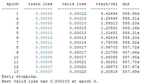
I used early stopping to help reduce overfitting:

class EarlyStopping(object):
 def __init__(self, patience=100):
   self.patience = patience
   self.best_valid = np.inf
   self.best_valid_epoch = 0
   self.best_weights = None

def __call__(self, nn, train_history):
 current_valid = train_history[-1]['valid_loss']
 current_epoch = train_history[-1]['epoch']
 if current_valid < self.best_valid:
   self.best_valid = current_valid
   self.best_valid_epoch = current_epoch
   self.best_weights = nn.get_all_params_values()
 elif self.best_valid_epoch + self.patience < current_epoch:
   print('Early stopping')
   print('Best valid loss was {:.6f} at epoch {}.'.format(
   self.best_valid, self.best_valid_epoch))
   nn.load_params_from(self.best_weights)
   raise StopIteration()

Step 3: Read the Training Data

As well as reading the training data, I shuffled the order of the data. This allowed me to use batch training.

# read the training data

printQ('reading the training data')
train_x, train_y, train_id = load_train_set()

printQ ('shuffling training rows')
random.seed(1234)
rows = random.choice(arange(0, train_x.shape[0]), train_x.shape[0])
t_x = train_x[rows,:,:,:]
t_y = train_y[rows,:]
t_id = train_id[rows]

printQ('finished')

Step 4: Train the Model

The network architecture used deep convolutional layers to find features in the image, then fully connected layers to convert these features into the centroid location:

# fit the models

# set up the model
printQ ('setting up the model structure')
layers0 = [
 # layer dealing with the input data
 (InputLayer, {'shape': (None, 2, 96, 96)}),

# first stage of our convolutional layers
 (Conv2DLayer, {'num_filters': 32, 'filter_size': 5}),
 #(DropoutLayer, {'p': 0.2}),
 (Conv2DLayer, {'num_filters': 32, 'filter_size': 3}),
 #(DropoutLayer, {'p': 0.2}),
 (Conv2DLayer, {'num_filters': 32, 'filter_size': 3}),
 #(DropoutLayer, {'p': 0.2}),
 (Conv2DLayer, {'num_filters': 32, 'filter_size': 3}),
 #(DropoutLayer, {'p': 0.2}),
 (Conv2DLayer, {'num_filters': 32, 'filter_size': 3}),
 (MaxPool2DLayer, {'pool_size': 2}),
 (DropoutLayer, {'p': 0.2}),

# second stage of our convolutional layers
 (Conv2DLayer, {'num_filters': 64, 'filter_size': 3}),
 #(DropoutLayer, {'p': 0.3}),
 (Conv2DLayer, {'num_filters': 64, 'filter_size': 3}),
 #(DropoutLayer, {'p': 0.3}),
 (Conv2DLayer, {'num_filters': 64, 'filter_size': 3}),
 (MaxPool2DLayer, {'pool_size': 2}),
 (DropoutLayer, {'p': 0.3}),

# two dense layers with dropout
 (DenseLayer, {'num_units': 128}),
 (DropoutLayer, {'p': 0.5}),
 (DenseLayer, {'num_units': 128}),

# the output layer
 (DenseLayer, {'num_units': 2, 'nonlinearity': sigmoid}),
]

printQ ('creating and training the networks architectures')
numNets = 1
NNs = list()
for iNet in arange(numNets):
 nn = NeuralNet(
 layers = layers0,
 max_epochs = 2000,
 update=adam,
 update_learning_rate=0.0002,
 regression=True, # flag to indicate we're dealing with regression problem
 batch_iterator_train=BatchIterator(batch_size=100),
 on_epoch_finished=[EarlyStopping(patience=10),],
 train_split=TrainSplit(eval_size=0.25),
 verbose=1,
 )
 result = nn.fit(t_x, t_y)
 NNs.append(nn)

printQ('finished')

Based upon how quickly the training converged, the network could possibly have been simplified, reducing the number of layers, or using fewer neurons in the fully connected layers. But I didn’t have time to experiment with different architectures.

The GPU quickly ran out of RAM unless I used the batch iterator. I found the batch size via trial and error. Large batch sizes caused the GPU to run out of RAM. Small batch sizes ran much slower.

Step 5: Review the Training Errors

Just like humans, all models make mistakes. The heart chamber segmentation algorithms I used later in this project were sensitive to how well the heart chamber was centred in the image. But as long as the model output was a centroid that was inside the heart chamber, things usually went OK. Early versions of my model made mistakes that placed the centroid outside the heart chamber, sometimes even far away from the heart.Tweaks to the training data (especially enhancing the data with rotation and reflection) and the architecture (especially dropout layers) improved the performance.

def getHeartLocation(trainX):
  # get the heart locations from each network
  heartLocs = zeros(numNets * trainX.shape[0] * 2).reshape((numNets, trainX.shape[0], 2))
  for j in arange(numNets):
    nn = NNs[j]
    heartLocs[j, :, :] = nn.predict(trainX)

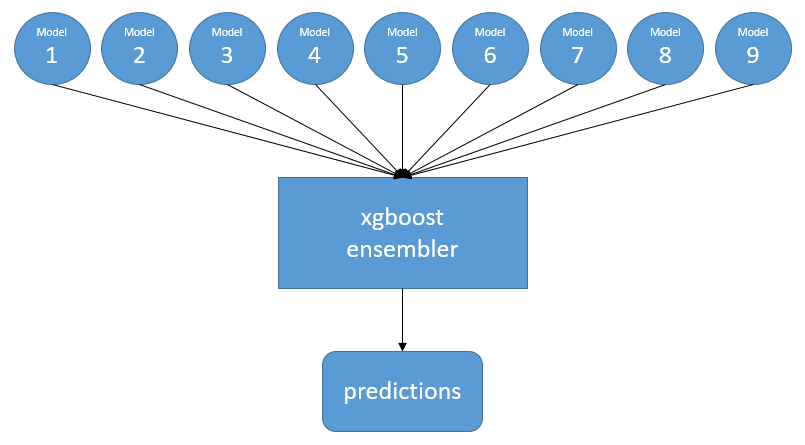
    # use median as an ensembler
    heartLocsMedian = zeros(trainX.shape[0] * 2).reshape((trainX.shape[0], 2))
    heartLocsMedian[:,0] = median(heartLocs[:,:,0], axis = 0)
    heartLocsMedian[:,1] = median(heartLocs[:,:,1], axis = 0)

    # use a 'max distance from centre' ensembler
    heartLocsDist = zeros(trainX.shape[0] * 2).reshape((trainX.shape[0], 2))
    distance = abs(heartLocs - 0.5)
    am0 = distance[:,:,0].argmax(0)
    am1 = distance[:,:,1].argmax(0)
    heartLocsDist[:,0] = heartLocs[am0, arange(trainX.shape[0]), 0]
    heartLocsDist[:,1] = heartLocs[am1, arange(trainX.shape[0]), 1]

    # combine the two using an arithmetic average
    heartLocations = 0.5 * heartLocsMedian + 0.5 * heartLocsDist

    return heartLocations

heartLocations = getHeartLocation(train_x)

# review the training errors to check for model improvements
def plot_sample(x, y, predicted, axis):
  img = x[0, :, :].reshape(96, 96)
  axis.imshow(img, cmap='gray')
  axis.scatter(y[0::2] * 96, y[1::2] * 96, marker='x', s=10)
  axis.scatter(predicted[0::2] * 96, predicted[1::2] * 96, marker='x', s=10, color='red')

nTrain = train_x.shape[0]
errors = np.zeros(nTrain)

for i in arange(0, nTrain):
  errors[i] = sqrt( square(heartLocations[i, 0] - train_y[i, 0]) + square(heartLocations[i, 1] - train_y[i, 1]) )

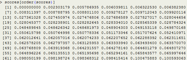
print('Prob(error > 0.05)' + str(mean(errors > 0.05)))
print('Mean: ' + str(mean(errors)))
print('Percentiles: ' + str(percentile(errors, [50, 75, 90, 95, 99, 100])))

for i in arange(0, nTrain):
  error = sqrt( square(heartLocations[i, 0] - train_y[i, 0]) + square(heartLocations[i, 1] - train_y[i, 1]) )
  if (error > 0.04):
    if train_id[i] != train_id[i-1]:
      #print(i)
      print(train_id[i]) # only errors on the original images - not the altered images
      fig = pyplot.figure(figsize=(6, 3))
      ax = fig.add_subplot(1, 2, 1, xticks=[], yticks=[])
      plot_sample(train_x[i,:,:,:], train_y[i, :], heartLocations[i, :], ax)
      pyplot.show()

print('error review completed')

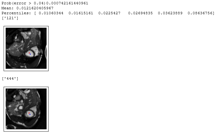
After many failed models, I was excited when the two worst training errors were still close to the centre of the heart chamber 🙂

Step 6: Find the Left Ventricle Locations for the Submission Data

The main point of building a heart finder machine learning model is to automate the process of finding the left ventricle in the test images that will be used as part of the competition submission. These are images that the model has never seen before.

def load_submission_set():
  numTimes = 2 # how many time periods to use
  plusTime = 5
  xs = []
  ys = []
  ids = []
  paths = []
  times = []
  saxes = []
  all_y = '/home/colin/data/Second-Annual-Data-Science-Bowl/working/centroids-submission-R.csv'
  with open(all_y) as f:
    rows = csv.reader(f, delimiter=',', quotechar='"')
    iRow = 1
    for line in rows:
      # first line is column headers
      if iRow > 1:
        # parse the line
        patient = line[0]
        x = 0
        y = 0
        sax = int(line[1])
        firstTime = int(line[2])
        # save the targets
        xy = np.asarray([x, y])
        ys.append(xy.astype('float32').reshape((1, 2)))
        # read the images
        folder = '/home/colin/data/Second-Annual-Data-Science-Bowl/validate-cleaned/' + patient + '/study/sax_0' + str(sax) + '/'
        xm = np.zeros([1, 2, 96, 96])
        #
        #
        # current frame
        path0 = folder + 'image-' + ('%0*d' % (2, firstTime)) + '.png'
        img = load_image(path0)
        # transform the image - rotation, reflection etc
        #img = transform_image(img, row['equalise'], row['gammaAdjust'], row['reflection'], row['rotation'])
        # get the pixels into the range [-1, 1]
        img = (img / 128.0 - 1.0).astype('float32').reshape((96, 96))
        xm[0, 0, :, :] = img
        #
        #
        # find movement of current frame to future frame
        path5 = folder + 'image-' + ('%0*d' % (2, firstTime + plusTime)) + '.png'
        img = load_image(path5)
        # transform the image - rotation, reflection etc
        #img = transform_image(img, row['equalise'], row['gammaAdjust'], row['reflection'], row['rotation'])
        # get the pixels into the range [-1, 1]
        img = (img / 128.0 - 1.0).astype('float32').reshape((96, 96))
        # first time is the complete image at time 1
        # subsequent frames are the differences between frames
        xm[0, 1, :, :] = img - xm[0, 0, :, :]
        xs.append(xm.astype('float32').reshape((1, numTimes, 96, 96)))
        ids.append(patient)
        paths.append(path0)
        times.append(firstTime)
        saxes.append(sax)
      iRow = iRow + 1
  return np.vstack(xs), np.vstack(ids), np.vstack(paths), np.vstack(times), np.vstack(saxes)

printQ('reading the submission data')
test_x, test_ids, test_paths, test_times, test_sax = load_submission_set()

printQ('quot;getting the predictions')
predicted_y = getHeartLocation(test_x)

printQ('creating the output table')
fullIDs = []
fullPaths = []
fullX = []
fullY = []
fullSax = []
fullTime = []
nTest = test_x.shape[0]
iTime = 1
for i in arange(0, nTest):
  patient = (test_ids[i])[0]
  sax = int((test_sax[i])[0])
  path = (test_paths[i])[0]
  iTime = int((test_times[i])[0])
  fullIDs.append(patient)
  fullPaths.append(path)
  fullX.append(predicted_y[i, 0])
  fullY.append(predicted_y[i, 1])
  fullSax.append(sax)
  fullTime.append(iTime)
  outPath = '/home/colin/data/Second-Annual-Data-Science-Bowl/predicted-heart-location-submission/'
  outPath = outPath + patient
  outPath = outPath + '-' + str(sax)
  outPath = outPath + '-' + str(iTime) + '.png'
  img = load_image256x192(path)
  x = int(round(predicted_y[i, 0] * 192))
  y = int(round(predicted_y[i, 1] * 256))
  img[y, x] = 255
  img[y-1, x-1] = 255
  img[y-1, x+1] = 255
  img[y+1, x-1] = 255
  img[y+1, x+1] = 255
  write_image(img, outPath)

fullIDs = array(fullIDs)
fullPaths = array(fullPaths)
fullX = array(fullX)
fullY = array(fullY)
fullSax = array(fullSax)
fullTime = array(fullTime)

printQ('saving results table')
d = { 'patient': fullIDs, 'path' : fullPaths, 'x' : fullX, 'y' : fullY, 'iTime' : fullTime, 'sax' : fullSax}
import pandas as pd
d = pd.DataFrame(d)
d.to_csv('/home/colin/data/Second-Annual-Data-Science-Bowl/working/heartfinderV4b-centroids-submission.csv', index = False)

In the animated gif below, you can see the left ventricle centroid location that has been automatically fitted, displayed as a dark rectangle moving around near the centre of the heart chamber. The machine learning algorithm was not trained on this patient’s images – so what you see here is artificial intelligence in action!